Deploying Trustworthy AI in the Courtroom: Lessons from Examining Algorithm Bias in Redistricting AI

I. Introduction

The inexorable advance of AI1 has achieved broad societal reach, including into the law. Over the last decade, the courts have reviewed novel forms of evidence enabled by new technological advances. This trend will likely not slow or reverse course in the future. Given the judiciary’s general lack of technical expertise, the potential for technological advances to create unintended difficulties for judicial decision-making seems likely. Thus, there needs to be a serious discussion about how the legal system should adapt to meet these inevitable changes.

Although the courtroom is in many ways a unique setting it faces similar challenges to those that other societal sectors are grappling with. Technological developments come rapidly and require nimble adaptation by society. We should consider the ramifications of, say, the metaverse and deep fakes before they become menacing rather than after. It would be naïve to believe that the courtroom will be spared from the ramifications of rapidly rising technological sophistication. Minimizing deleterious effects on the justice system requires learning from what we know so far and being proactive about experimenting with solutions.

In this Article, we focus on the legal landscape surrounding electoral redistricting. We begin by explaining the general concept of algorithm bias. We then describe how this conception of algorithm bias emerges in redistricting litigation. Finally, we propose avenues for mitigating the deleterious impact of algorithm bias in this legal arena and comment on general lessons learned from this context for deploying trustworthy AI in the courtroom.

II. Algorithm Bias

The increasing deployment of algorithms for societal decision-making has been met with both enthusiasm for its potential and criticism for its lack of transparency and its capacity to generate unfair and indefensible results. There is considerable concern about the harmful impact of “algorithm bias.” The precise definition of algorithm bias is unclear, but generally it means that an algorithm leads to decisions that are either incorrect or systematically unfair to a particular group.

Consider facial recognition algorithms that seek to identify people based on their facial features. These algorithms can be used to unlock a cell phone as well as for criminal surveillance. If an algorithm fails to unlock your cell phone, the misidentification or lack of identification presents the minor inconvenience of then needing to type in a passcode. When facial recognition algorithms are used for police surveillance, customs screening, or employment and housing decisions, however, inaccurately assessing biometrics can lead to more serious consequences: improper criminalization, perpetuating inequality, or an inequitable distribution of public benefits.

Although law enforcement issues have received the most media attention, there are many potentially harmful applications. Beyond simple facial recognition, algorithms can also be used to identify verbal and nonverbal cues through facial movements and/or speech patterns to rank job candidates on measures such as confidence and personality. Algorithms used to allocate patient health care to patients have sometimes assigned the same level of risk to White and Black patients even though the latter were sicker.2 There is evidence that Facebook ad-generation algorithms fuel societal polarization,3 and that school assignment algorithms for students can increase societal inequities.4 To be sure, algorithms can also efficiently and effectively produce desirable outcomes. Algorithms, for instance, have been used to take attendance in schools, monitor the sleepiness of drivers, and prevent unauthorized building access on college campuses.

In the legal context, AI can also help judges make better informed decisions by providing more information or new forms of evidence. But to achieve these desirable goals, we need to understand how to deploy trustworthy algorithms, which begins with understanding their pitfalls. “Algorithm bias” is multi-faceted, comprised of various components that are often conflated. In this Article, we aim to identify how specific forms of algorithm bias may affect legal decision-making by focusing on two aspects: data bias and lack of domain knowledge. While these are not the only forms of algorithm bias, we begin here with the idea that decreasing any facet of algorithm bias results in movement in a positive direction.

A.    Data Bias

Data bias is a widely recognized source of “algorithm bias.” It can, for example, result from training a facial recognition algorithm on only white faces, in which case the algorithm will almost certainly identify light-skinned faces more accurately than dark-skinned faces. In this case, while the algorithm itself may be capable of accurately distinguishing nonwhite faces, it has not been trained to do so. A study by the National Institute of Standards and Technology (NIST) that included an examination of 189 facial recognition algorithms found that Asian and Black faces were 10 to 100 times more likely to be falsely identified than White faces, women were falsely identified more than men, and Black women were misidentified most often.5 Similarly, the top three gender classification algorithms appear to have difficulties identifying women, especially darker-skinned females.6 In a number of these instances, there are selection bias issues—although the data that are used to train the algorithm are not representative of the larger population, inferences for the entire population are still made from these limited data. In the election law realm, danger lurks because there are potential gains to expert witnesses who use data selectively to advance the arguments that lawyers who hire them want to advance.

B.    Domain Knowledge

Algorithm bias can also arise when the use of an algorithm is proposed but without sufficient domain knowledge. An example of insufficient domain knowledge in facial recognition algorithms would be an algorithm written by a person who has neither studied nor understands the characteristics of distinguishing facial landmarks. Indeed, the relevant facial features to measure and how these measures are then combined to identify a face are determined, not from knowledge of math or computer science, but from domain knowledge. That is, one needs to understand the fundamental components of a face (structure, skin color, etc.) to know how to properly code a facial recognition algorithm. If these fundamental components are not captured, then the algorithm, notwithstanding advances from computer science or statistics, will perform poorly (or in a biased manner). Even when the underlying mathematics are pristine, if domain knowledge is poorly understood or integrated, the AI models will perpetuate this lack of understanding, creating another form of “algorithm bias.”7 In the legal field, considerable domain knowledge is required since what is relevant to measure is determined by case law and must fit into a legal framework. Mathematicians and computer scientists can create algorithms, but neither they nor their algorithms create law. They create measures. Judges create standards.

III. Data Bias in Redistricting AI

In the last decade, new algorithms, and measures such as the Efficiency Gap (EG) have been proposed and presented as evidence in redistricting litigation. EG is a simple calculation that is intended to provide a measure of the difference in “wasted votes” between two political parties.8 In an exchange about EG, Justice Roberts commented,

[I]f you’re the intelligent man on the street and the Court issues a decision, and let’s say, okay, the Democrats win, and that person will say: “Well, why did the Democrats win?” And the answer is going to be because EG was greater than 7 percent, where EG is the sigma of party X wasted votes minus the sigma of party Y wasted votes over the sigma of party X votes plus party Y votes.

And the intelligent man on the street is going to say that’s a bunch of baloney. . . . [Y]ou’re going to take these—the whole point is you’re taking these issues away from democracy and you’re throwing them into the courts pursuant to, and it may be simply my educational background, but I can only describe as sociological gobbledygook.9

EG is a highly flawed measure,10 but it was clear that Justice Roberts neither understood its technical flaws in any detail nor how it could be relevant to a legal framework. Perhaps, he is also just generally suspicious of expert testimony.11 Whatever the origins of Roberts’s comment, however, caution about new technical innovations is appropriate and each innovation deserves proper scrutiny. Most measures and algorithms will have drawbacks and advantages. There is no general solution to “algorithm bias,” but we can analyze how it has been used to date in redistricting litigation with the hope of clearing up potential confusions and suggesting ways to enable a more trustworthy deployment of AI in the courtroom.

A.    Data Bias

Data bias issues apply to all AI tools since algorithms detect patterns from the data they are given. Unsurprisingly, redistricting AI is no different in this respect. To illustrate the critical role of data choices in redistricting algorithms, consider these three examples that hail from academic literature and expert evidence presented in redistricting litigation.

1.     Example 1: Partisan gerrymandering of Florida’s congressional districts

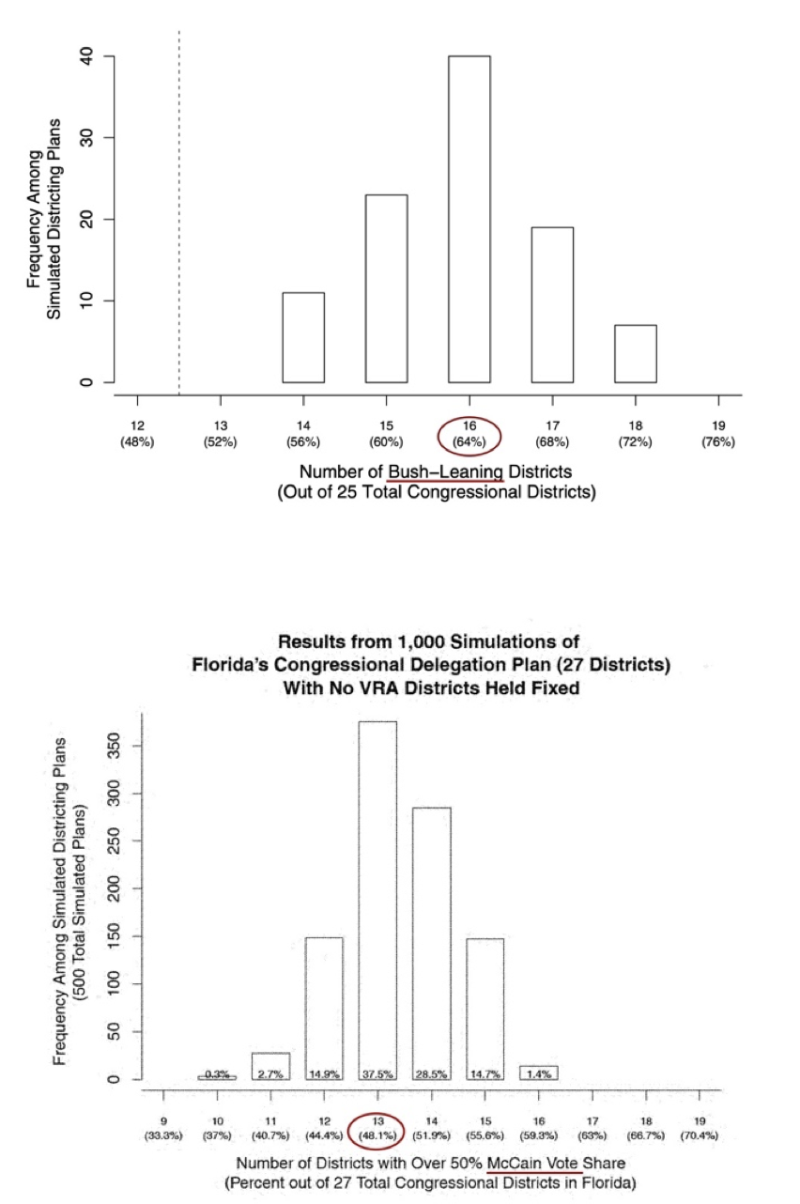
In a 2013 Quarterly Journal of Political Science article, Chen and Rodden argue that “in many states, Democrats are inefficiently concentrated in large cities and smaller industrial agglomerations such that they can expect to win fewer than 50% of the seats when they win 50% of the votes.”12 They “show that in many urbanized states, Democrats are highly clustered in dense central city areas, while Republicans are scattered more evenly through the suburban, exurban, and rural periphery.” They then demonstrated this pattern with an in-depth case study of Florida.13 Their analysis included hundreds of “random simulations”14 of congressional district maps for Florida where the “Republicans won an average of 61% of the seats. The most biased of the simulated plans gave the Republicans 68% of the seats, and the least biased plan gave them 56%.”15 This result leads them to conclude that there exists a “significant pro-Republican bias that results from a districting procedure that is based solely on geography and population equality. Moreover, this result is not driven by the compactness of the simulated districts. The results are just as striking when we use the non-compact simulation procedure.”16 They further examined the actual plan enacted by the Republican-controlled Florida legislature in 2002 and found that it fell within their distribution. Thus, they conclude that, “because the enacted districting plan falls within the range of plans produced by our compact districting procedure, we are simply unable to prove beyond a doubt that the enacted districting plan represents an intentional, partisan, Republican gerrymander.”17

In their study, they measure partisanship using the Bush-Gore 2000 presidential election. They state that “[f]or each of these simulated districting plans, we calculate the Bush-Gore vote share of each simulated single-member district, and we use this vote share to determine whether the district would have returned a Democratic or Republican majority.”18 They chose to use the 2000 presidential election data to assess partisanship “because of its unique quality as a tied election.”19

In the same year as their published paper, the authors served as expert witnesses for Florida’s gerrymandering case.20 For that work, they describe the identical simulation procedure for Florida’s congressional districts. To analyze partisanship for litigation, however, they switched from the Bush-Gore 2000 election that they used in their published article to the Obama-McCain 2008 presidential election.21 Since McCain received 48.6% of the two-party vote in Florida in 2008 while Bush captured 50% of the vote in 2000, the number of Republican votes (and thus their assessment of who is a “Republican”) declined. If there are fewer Republicans, then it is more difficult to draw “Republican districts.” While the QJPS paper had placed the modal number of Republican leaning districts at 16/25 (64%), the expert report for litigation placed the modal number of Republican leaning districts at 13/27 (48.1%).22 In addition, while the published paper reported that the simulations were unable to produce a single districting plan that was neutral or pro-Democratic in terms of electoral bias, the simulations for litigation very commonly produced pro-Democratic plans. Their expert report then, in direct opposition to their published journal article where they were unable to prove beyond a doubt that the enacted districting plan was a Republican gerrymander, concluded that the Florida congressional districts constituted a partisan gerrymandering.

Figure 1

They defended the data switch in a supplementary report by saying that the

initial decision to use the presidential vote was based not only on a desire for continuity with our earlier work, where the presidential vote was our only option to facilitate cross-state comparisons, but also on our assessment that it was the `cleanest’ available measure of partisanship that would allow us to aggregate up to the level of simulated (and enacted) Congressional districts and make inferences about which party would obtain a majority of those districts.25

Whether this is a good and defensible reason is outside the scope of this Article. Since the published article was completed in 2012 and the expert report was written in 2013, both the 2000 Bush/Gore data and the 2008 Obama/McCain data were available for both the scholarly work as well as the expert report. To be clear, we are making no claims about who did or did not gerrymander or how many districts truly lean Republican or Democrat in Florida. We are simply noting that data choices matter when making partisan assessments, and that these decisions can, in fact, be the pivotal decisions in a partisan gerrymandering analysis.

2.     Example 2: Partisan gerrymandering of Massachusetts’s congressional districts

Duchin et al. (2019) examine congressional redistricting in the state of Massachusetts and claim that “[t]hough there are more ways of building a valid districting plan than there are particles in the galaxy, every single one of them would produce a 9-0 Democratic delegation.”26 This is a large claim, and one that is necessarily based on knowledge of how many Republicans and how many Democrats are in the state and where these partisans reside. Duchin et al. examined partisanship data in the form of precinct returns for “election results from 13 presidential and US Senate elections in Massachusetts.”27 These election returns are shown in the first 13 entries of Table 1, which are replicated from their article (with red highlights added to indicate races that were won by Republicans).

Table 1. Select Statewide Two-party Election Returns in Massachusetts (2000-2020).

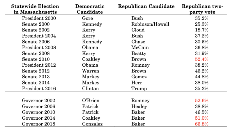
Of course, there are other elections in this time period, which Duchin et al. duly acknowledged: “[t]he analysis could certainly be extended to other statewide races, including governor, attorney general, and secretary of state as desired; we chose a collection of races that demonstrates interesting distributional effects in the 30%–40% range of Republican share” (emphasis added).28 The authors do not mention, however, that their “data choice” has substantive consequences.29 Consider the five entries at the bottom of Table 1 which show the statewide Governor’s race for the same time period, a statewide race that certainly could have been included in their analysis, but was not one that they chose. Interestingly, while the state of Massachusetts regularly favors Democrats in Presidential and US Senate elections, it has, in the same period, more often elected a Republican Governor than a Democratic Governor. More recently, it has done so with overwhelming margins, such that it is the Democratic candidate who is in the 30 to 40 percent vote range in these races.

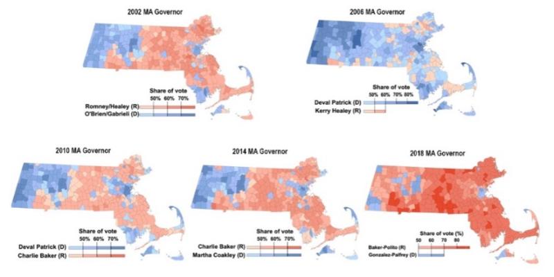
Duchin et al. use their curated data to demonstrate that with the resulting geographical distribution of partisans, it is impossible to assemble a congressional district in which Republicans were the majority. Figure 3 replicates their figure that shows this result visually. The map on the left shows the 2000 Bush v. Gore race by towns, and the map on the right shows the 2006 Chase v. Kennedy race by precinct. Contrast this with Figure 4 that shows strong Republican contingencies in the Governor’s races from 2002–2018. These visuals imply a markedly different set of partisan preferences. To be clear, we are not proposing that one should determine partisanship from the Governor’s races or that the Governor’s races matter more or less than other statewide elections. We present these visuals simply to demonstrate the impact of data choices.

Figure 3

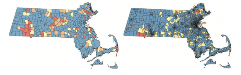
 Figure 4

We in no way deny that it may be defensible to use some election results and not others, but such a defense should exhibit strong domain knowledge and serious contemplation of the electoral dynamics in the state of Massachusetts. Duchin et al., instead, state that

[m]any political scientists have debated whether statewide races are good predictors of congressional voting patterns, and if so, which ones are most predictive. That debate is beside the point for this analysis, which is focused on the range of representational outcomes that are possible for given naturalistically observed partisan voting patterns.30

What “naturalistically observed partisan voting patterns” means is unclear since an election as important as the statewide Governor’s race seem as natural, observed, and partisan as any election in the state.

It may be that Duchin et al. are simply studying “the extent to which empirical patterns in actual voting data can restrict the range of representation that is possible for a group in the numerical minority.”31 That would be fine as a theoretical study, and we certainly concur that it is difficult to obtain representation when one’s group is a numerical minority, and may be impossible if the minority is spread in a sufficiently geographically uniform manner across the state. This is not a novel discovery, but has, instead, long been known about the single member districting scheme in the American political system.32 However, the Duchin et al. article goes well beyond a strictly theoretical claim and unequivocally argues “that the underperformance of Republicans in Massachusetts is not attributable to gerrymandering, nor to the failure of Republicans to field House candidates, but is a structural mathematical feature of the actual distribution of votes observable in some recent elections.”33 Indeed, not one sentence in the abstract of the paper focuses on a purely theoretical claim while the substantive claims are central and clear.

A slightly deeper dive with the data indicates that the implications are more nuanced. While Massachusetts appears to be quite a strong Democratically leaning state, candidates and campaigns do apparently matter. These Democratically inclined voters in 1984, voted for Ronald Reagan (51.2%) over Walter Mondale, and they have recently supported a Republican more often than a Democrat to serve as their Governor. Hence, the claim that gerrymandering does not matter is not clear. If a district is drawn in such a way that it is overwhelmingly comprised of Democrats, then it is less likely that the Republicans will field a candidate and even less likely that they will field a quality candidate. On the other hand, when a quality candidate runs, there is ample evidence that Massachusetts voters are not blinded by partisanship, but are, instead, intelligent voters who are willing to vote for the candidate they deem is best, party notwithstanding.

Again, we wish to clearly state that we are not making any claims about whether gerrymandering is or is not occurring in Massachusetts. We wish only to draw attention to the point that the data choices are important and can be pivotal.

3.     Example 3: Partisan gerrymandering of Ohio’s congressional districts

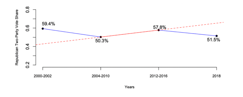
For the 2018 Ohio congressional redistricting litigation, Cho calculated the average Democratic vote share using data from the 2008–2010 contested and competitive statewide elections.34 These data were chosen because they were the most proximate to the redistricting and thus would have been the data available and used by the map drawers.35 In rebuttal, an expert from the defense claimed that “[t]he state-level partisan vote index for the 2004 to 2010 time period registered 50.3% Republican. For the 2012 to 2016 period, the statewide partisan index was 57.8% Republican, an increase of 7.5-points.”36 The implication is that the number of Republicans in Ohio is on an upward trajectory, and that it is this partisan trend, not necessarily the redistricting map, that accounts for the Republican victories in the state. However, regardless of whether Ohio had become more Republican since the 2010 redistricting or not, an analysis of the enacted map should not be assessed with data that was not available to the map drawers.

In addition, the point about data is misleading in another way. Judging the partisanship of Ohio by drawing a line between two curated data points and then extrapolating outside that time frame does not give a full picture of changing partisan votes in the state. Figure 5 shows that while there was an “increase in Republicans” in the 2004–2016 period, adding the pre-2004 and post-2016 data points changes the picture dramatically. The implied upward trajectory disintegrates.

Figure 5

Again, as in the two previous examples, we see clearly that data choices are highly consequential in the assessment of the substantive claims. The data choices are wholly separate and can change the conclusions drawn from the statistical models or computer simulations. “Data bias” is not particular to one political party’s analyses. There is copious evidence that this type of “data bias” happens in analyses produced on both sides of the partisan aisle.

B.    Data Solutions: Instituting a Set of Standards for Best Practices

Evidently, “data bias” in redistricting AI is as much of a concern for redistricting as it is for any other AI application. The ability to craft outcomes by carefully choosing data sets is indisputably problematic. Reducing this form of “algorithm bias” is essential for deploying trustworthy AI in the court room. Political scientists have long known that assessing partisanship is not simple. This is why political scientists have developed the concept of the “normal vote.”38 The normal vote is rooted in a conception of elections being subject to short-term and long-term forces. The former includes regional swings to and from given parties on the basis of timely issues as well as district-level forces particular to given elections. Prominent in this latter category are any candidate effects, such as an incumbency advantage or a friends-and-neighbors advantage a candidate enjoys in his hometown or region. The major long-term determinant of election returns is the normal vote, the expected breakdown of vote shares when the parties field comparable candidates and election-specific effects are controlled for.

While it is not simple to measure normal partisanship levels, creating a partisanship measure is also not a futile endeavor. At minimum, one way to ameliorate issues with cherry-picking data is to institute a set of standards for best practices. The rise in technology can certainly have a positive effect here. It is now simple to create and maintain data repositories. It is also relatively simple to create online communities that can cross check and improve data quality. For instance, the Redistricting Data Hub has already created a data repository for redistricting.39 Their data repository does not need to be the central or only repository, but it minimally demonstrates concept feasibility. It is also feasible to score and check the data quality via crowd sourcing. Precinct-level election data are now widely available. The past excuses that only select data were available are no longer defensible.

A movement toward a “best practices” solution might involve deriving a “default” measure of partisanship that would be comprised of, say, all statewide races for the last two election cycles. Researchers or expert witnesses could then use this measure, or, if they felt that the conditions (strong incumbency effects or non-competitive elections) compelled them to deviate from the default measure, they would be required to explain how and why, with a showing of the results from using the default set of elections as well as their modified set of elections. The courts might also develop a strong norm or rule that the results from a range of statewide outcomes are presented, which would help judges understand how robust the results are to competitive districts or possible swings from election to election. Alternatively, or in addition, a particular set of data could be “pre-approved” by both sides through an adversarial process. Elsewhere we suggest changes to the structural framework of legal decisions that are also helpful for alleviating data bias issues.40

Instituting standard practices is straightforward and would be a highly effective way to address the “data bias” issue in redistricting. Multiple and reinforcing mechanisms are possible. Although these practices would be novel for litigation, as data becomes increasingly prevalent for decision-making in all walks of life, it behooves the court to institute structural safeguards to avoid the negative externalities before they worsen.

IV. Reducing the “Gobbledygook” for the Judiciary

“Data bias” is but one form of “algorithm bias.” Algorithm bias may also occur when there is a mismatch or miscommunication between the technical and legal communities. Employing algorithms in a legal setting is challenging partly because of the difficulty in communication that arises from the confluence of technical and non-technical communities. Here, “algorithm bias” may arise from either a lack of technical understanding by lawyers and judges or by a lack of domain knowledge by those who propose the algorithms. Apropos this point, we have commented that

[l]egal questions cannot be decided by mathematicians. Mathematicians may make proposals, but judges decide whether to accept those proposals . . . judges must clearly understand the mathematical concepts (even if not the mathematical details) to make a reasoned judgment. However, when the science is unclear, we have only miscommunication, from which no one benefits.41

To be sure, “mathematics” and “algorithms” are not inherently useful and even harmful when misunderstood or mis-applied. This issue—that the justices do not understand how algorithms sit within a rigorous legal framework (and relatedly that the algorithms are not being described correctly)—is the heart of “sociological gobbledygook.”

A.    Partisan Gerrymandering

The Court is aware of the curious irony created by its separate decisions on partisan and racial gerrymandering:

an excessive injection of politics is unlawful. So it is, and so does our opinion assume. That does not alter the reality that setting out to segregate voters by race is unlawful and hence rare and setting out to segregate them by political affiliation is (so long as one doesn’t go too far) lawful and hence ordinary.42

In the landmark partisan gerrymandering case, Rucho v. Common Cause,43 the Court ruled that while partisan gerrymandering is unconstitutional, there was no judicially manageable standard that could be used by the Court to assess the extent of partisanship used to construct an electoral map. There were many computer-simulated maps offered as evidence that the enacted map being litigated in Rucho was excessively partisan. However, the Justices were confused about how the algorithmic evidence could help them to define a legal standard of excessive partisanship:

JUSTICE ALITO: No, no, but can you just answer that -- that question, because it’s a real puzzle to me. So you’ve got -- let’s say you’ve got 100 maps or you might even have 25. I think you probably have thousands. So you have all of these maps, and you have to choose among them. The legislature chooses among them. And you’ve already programmed in all of the so-called neutral criteria. How do you -- how does the legislature go about choosing among those maps? Would anything other than just random choice be sufficient -- be satisfactory?

MR. BONDURANT: The legislature has wide discretion, as long as it does not attempt to do two things: dictate electoral outcomes, favor or disfavor a class of candidates. That is an easily administered --

JUSTICE GORSUCH: But, counsel, that -- that first one, dictate electoral outcomes, I think is going to turn -- turn on -- on numbers, right? How much deviation from proportional representation is enough to dictate an outcome?

So aren’t we just back in the business of deciding what degree of tolerance we’re willing to put up with from proportional representation? We might pluck a number out of the air or see that, you know, maybe two-thirds is used for veto overrides, so we like that. Where -- where are we going to get the number on the business end of this?

MR. BONDURANT: The business end of it is looking at how this is done. This was done by looking at voting history as the best predictor of voting behavior. Sorting voters among districts to achieve a particular outcome, to guarantee that in 10 districts, there would be safe Republican majorities in which the general election is essentially irrelevant and the primary election is the determining factor.

JUSTICE ALITO: Well, let me try one more time. So we’ve got  -- let’s say that you have a range of outcomes with all of these neutral maps that satisfy the neutral criteria, and they extend from 10 to two in favor of Republicans to 10 to two in favor of Democrats. So which one do you choose -- do you have to choose? Nine to three for Republicans? Eight to four? Six to six?

MR. BONDURANT: The -- the -- clearly, it’s an evidentiary matter in terms of intent. If the predominant intent is to favor one party, to penalize another based on their voting history, that goes too far, but --

JUSTICE KAVANAUGH: Isn’t that always going to be the case when you deviate too far from six to six, in Justice Alito’s hypothetical?

MR. BONDURANT: It certainly is going to be a question of factual proof. The closer you come to proportional representation, the harder it’s going to be for a plaintiff to prove that there was an intent.

JUSTICE GORSUCH: Well, there we go. I think that’s the answer to the question, right? Is that we’re going to -- that your -- you would like us to mandate proportional representation.

MR. BONDURANT: Not at all. Our position is you cannot discriminate intentionally against political parties and voters based on their political views and their voting history.

JUSTICE GORSUCH: And the further you deviate from proportional representation, the more likely you are to be found guilty of that.

MR. BONDURANT: It is purely an evidentiary question. This Court itself said in Reynolds, it said again in LULAC, that in a case in which you look statewide and see proportional representation, it is less likely . . . that you have gerrymandering.44

The Court raises two issues. First, the large number of simulated electoral maps from the algorithm is difficult to separate from notions of proportional representation (PR), which the Court has already rejected. The second problem involves the wide discretion given to legislatures in devising their electoral maps that permits them to use partisan and other political information and restricts only “excessive partisanship.”45 The Court is confused about how an algorithm that created a set of non-partisan maps is consistent with the wide discretion given to legislatures that permits them to use some partisan information. Mr. Bondurant, in reply, does not distinguish the algorithm-produced non-partisan maps from proportional representation and does not explain how to maintain wide discretion for the legislature. The inability to explain how the technological evidence fits within the legal framework is obviously problematic. Note here that what the justices find insufficient is the legal argument that integrates the technical evidence, not a technical argument explaining how the algorithm works. How might an algorithm that produces a non-partisan set of maps be relevant to a partisan gerrymandering claim?

On the proportional representation question, while the justices understand that non-partisan maps exhibit a range of partisan outcomes, they do not comprehend how to use them to identify a partisan gerrymander. Mr. Bondurant responds to the confusion, not by uncoupling the computer-generated maps from PR, but by discussing what factual proof is necessary depending on how close you are to PR. The critical distinction is between clustering effects that result from following formal criteria such as compactness, contiguity, and respect for local jurisdiction boundaries. These computer-drawn maps did not use political data. They are instead generated according to the locations of the state’s residents and formal map-drawing criteria. Hence, they display the range of possible partisan outcomes if the map is constrained only by minimum thresholds of those criteria.

If partisans are randomly dispersed in roughly equal numbers throughout the state, proportional outcomes would be a “natural” (i.e., not politically constructed”) outcome. When party voters cluster geographically in nonrandom ways, it can undermine “natural” seat-vote proportionality. The size of the discrepancy from proportionality depends on the degree and nature of partisan clustering. An over-concentration or over-dispersion of one party can yield a smaller than proportionate seat share for one party and a larger one for the other. But politically motivated clustering can sometimes promote more proportional outcomes as was the intent behind many Voting Rights Act Section 2 remedy plans that deliberately clustered historically under-represented communities in more favorable ways to ensure more equal opportunities for them.

A complete set of maps generated by adhering to the thresholds of legally defined formal criteria provides a baseline range of all possible political outcomes that occur without consideration of political data. The reason to simulate maps is to separate the effects of natural clustering from political clustering. It provides evidence of where a proposed map lies on the continuum of all possible maps with respect to not just likely partisan outcome but also for each of the formal criteria. Algorithmic evidence is not about achieving proportionality unless it is supplied with political data and programmed to search for such outcomes. Instead, it provides a context of how unusual or extreme a plan outcome is from the entire set of possible plan outcomes, and at what cost or detriment to formal criteria. It provides a basis for comparison and contextualization, but not a judicial determination for the courts.

A second issue is that the Elections Clause in the Constitution grants wide discretion to the states in devising its electoral maps, including the use of partisan information, so long as that use is not excessive. The argument by the challengers in Rucho is, in essence, that being on the tail of the distribution (i.e., producing an unusually uncommon partisan effect) is de facto evidence of the state overstepping its discretionary powers. The state, on the other hand, points out that all of the baseline maps have “partisanship taken out entirely,” and observes that “you get 162 different maps that produce a 10/3 Republican split” (i.e. far from proportional representation).46 Accordingly, all of these declaredly non-partisan maps, even the ones that are not close to PR, should fall within the legislature’s discretion. The dispute is about whether a plan that falls at the tails of the distribution from the baseline set of maps indicate “dictating outcomes” or within the legislature’s “discretionary powers.”

Indisputably, a state is not constrained to considering only neutral map-drawing principles: many decisions go into devising a map, and a state has wide latitude to act in the interest of its people. There are many non-partisan considerations that are outside the set of formal or “traditional districting principles.” One example is a claim about whether a community is better off with one or two representatives.47 Such a consideration is not partisan but is political in the sense that it concerns how best to garner greater political power. Whether the underlying intent is partisan or not, we leave aside. Without dispute though, it is a feature, not a flaw, for the legislature to have wide latitude to work in the interest of its people. Moreover, there can be many considerations beyond party that lie behind a particular map configuration. Possibly, a representative wants her church or her family’s cemetery in her district. Why a representative might want those things may be personal and completely devoid of partisan motivation. These types of decisions all fall within the wide latitude and discretionary power of the legislature to devise its electoral map.

Notice, however, that formal and political considerations, aside from pure party considerations, still have partisan effects. Every time a boundary is changed, partisans are shifted from one district to another district, necessarily altering the partisan balance.48 But, if non-partisan decisions have a partisan effect, how do we know if the admittedly many decisions behind a map make it “excessively partisan?” It would be impossible, almost surely, and impractical, at the very least, to try to discover whether each decision was intentionally partisan or not.

If the legislature acted like the redistricting algorithm and adhered only to the specified “neutral criteria,” the expected effect would mirror the baseline set of maps. But since the legislature is free to consider many other criteria, how is a baseline set of non-partisan maps relevant? When a legislature or even a redistricting commission draws district lines, it will intentionally make decisions with both formal and political considerations in mind (e.g. partisanship but also perhaps to help or hurt the electoral prospects of incumbents in either the primary or general elections). Consider that roughly half the time (with the exact probability depending on the political geography of the state), a non-partisan decision will shift partisans in a way that favors Republican interests. Roughly the other half of the time, it will shift partisans in a way that is advantageous to the Democrats. To be sure, every shift favors one party over the other.49 Each of these decisions, partisan or not, nonetheless changes the partisan effect of the map. However, the non-partisan decisions should have no systematic bias toward the Republicans or the Democrats, and so their collective partisan effect should wash out in the aggregate.

If the partisan effect of the enacted map is all the way on the right end of the distribution of partisan effect (i.e. an extreme partisan effect), that means we either began on the tail, which is extremely unlikely, or we started in a more likely spot and then the subsequent decisions moved that partisan effect to the end of the distribution. If the first “non-partisan decision” makes the map more Republican leaning, that is not bothersome since it must have some partisan effect. If the second “non-partisan decision” moves the map in the Republican direction again, that is also not so unusual. If the entire set of “non-partisandecisions” overwhelmingly favors the Republicans and moves the partisan effect all the way to the end of the distribution, we have strong evidence that those collective decisions were actually partisan in nature.

The legislature may also violate one or more of the lower bound thresholds of formal criteria. The non-partisan baseline set of maps provides context for assessing whether a plan is excessively partisan in the sense that it violates the other traditional formal state or federal criteria. Parallel reasoning has resulted in a tightening of deviations from the ideal population over time, especially for Congressional districts. There is a similar principle in Shaw and its progeny50 that placed a limit on extremely contorted, noncompact proposed majority-minority seats. Certainly, states could assist the court by more explicitly defining fair representation within state legislation or state constitutions. Absent such clarification, plans that favor one party intentionally but without serious sacrifice to formal criteria could also be judged as less “excessively partisan” than one that sacrifices other criteria for the sake of partisan advantage.

What constitutes “excessiveness” is a matter for the courts to decide. The purpose of baseline set of non-partisan maps is to situate a particular plan in terms of partisan effect and impact on traditional legal criteria. It serves as the empirical basis for a judicially manageable standard for assessing whether legislative decisions are excessively partisan that is consistent with the Constitution’s regard for states’ rights, honors the Elections Clause that provides wide latitude to the states to prescribe the times, places, and manner of its elections, supports our system of geographically based single member districts, bolsters the legislature’s mandate to legislate for the people, and is not dependent on notions of proportional representation. This result is achieved, not by the algorithm itself, but by combining the technological advancement with a rigorous legal argument that can arise only from strong domain knowledge of the law.

B.    Parallels and Dissimilarities Between Racial and Political Gerrymandering

Is the role of algorithmically drawn maps the same for racial gerrymandering cases? We maintain that while there are some similarities, there are important differences in the applicability of an algorithmically produced baseline set of maps for racial gerrymandering cases. From a pure measurement perspective, one could determine the level of natural clustering of racial groups given threshold values of formal criteria, which can also be done with partisan groups. Both types of cases pertain to the limits of designing districts to confer political advantage for one voter group over another. Both also involve measuring “excessiveness,” either with respect to partisanship or when race is the predominant factor in Voting Rights cases.

But there are important differences in how natural clustering is interpreted in the two types of cases that arises from the legacy and persistence of racism. City boundaries have been altered over time in many places through annexations to exclude non-White areas for reasons of racial prejudice or because some wealthier communities did not want to pay for city services that would support poorer populations. Redlining made it harder for Black voters to buy property in predominantly White areas, creating racial clustering by housing stock. Beyond redlining, disadvantaged groups almost by definition have more limited options with respect to finding affordable housing, which can result in ghettoization. And even when states pass requirements for local communities to provide low-income housing, the record of compliance can be uneven and minimal, at best, for NIMBY51 reasons.

Secondly, there are critical differences between the judicial framework of racial and partisan gerrymandering cases. In the former, the issue is typically to what degree can race be considered to remedy under-representation based on racial and ethnic prejudice. Race cannot intentionally be used to diminish the political representation of an underrepresented group. Where partisan rivalry is an inherent feature of a competitive democratic system, strong racial, ethnic or gender tensions can undermine democracies.52 Single member, simple plurality systems make governance easier and more stable by exaggerating the winning party’s shares beyond proportionality. Democracies are also allowed to discriminate against small parties by setting minimum vote thresholds to be automatically listed on the ballot. But our constitutional and statutory commitments to racial equality prohibit similar treatments based solely on a racial identity.53

This means that there is a different legal framework for interpreting a set of algorithmically created maps for racial gerrymandering cases. Computer-drawn maps based on formal criteria overlap to some degree with key aspects of a Section 2 analysis. The first prong of a Gingles test54 requires that a historically underrepresented group must be geographically compact and sufficiently large in population to have a chance of electing a representative of their choice. When groups are not sufficiently clustered and require very contorted district lines to provide an opportunity to elect, a districting plan is more prone to running afoul of Shaw limits on using race as a predominant factor.55

Today, the Court recognizes a new cause of action under which a State’s electoral redistricting plan that includes a configuration “so bizarre,” that it “rationally cannot be understood as anything other than an effort to separate voters into different districts on the basis of race [without] sufficient justification,” will be subjected to strict scrutiny.56

Race-based districting is subjected to strict scrutiny in the same way that any race-based law would. Minority districts created through a race-neutral AI process might be in a safer harbor from Shaw claims, but it does not follow that a race-neutral process is necessary to avoid strict scrutiny. In fact, racial consideration is necessary to some degree to remedy past discrimination.

The plaintiff in a racial gerrymandering case bears the burden of proving the unconstitutional usage of the race classification and may do so either through “circumstantial evidence of a district’s shape and demographics” (i.e. the district shape is so bizarre on its face that it is “unexplainable on grounds other than race”),57 through “more direct evidence going to legislative purpose,”58 or by showing a disregard for “traditional districting principles such as compactness, contiguity, and respect for political subdivisions. We emphasize that these criteria are important not because they are constitutionally required—they are not—but because they are objective factors that may serve to defeat a claim that a district has been gerrymandered on racial lines.”59 Miller v. Johnsonreiterates and clarifies that a legislature may be conscious of the voters’ races without using race as a basis for assigning voters to districts. The constitutional wrong occurs when race becomes the “dominant and controlling” consideration.60

For partisan gerrymandering, as explained earlier, the non-partisan baseline is relevant because it provides a basis for assessing the partisan effect of the myriad decisions that go into devising an electoral map. This is possible because whenever a geographic unit is reassigned, whether this decision is motivated by partisan considerations or not, a partisan effect necessarily ensues. However, while every shift of a geographic unit results in a partisan effect, every shift does not result in a racial effect. There are many shifts that are unrelated to the formation of a minority district. Since not every decision has a “racial effect,” the argument for the relevance of the non-partisan baseline does not translate to a relevance for a race-neutral baseline. The relevance of the race-neutral baseline is further unclear if it was not created with partisanship in mind since, presumably, partisan factors are also race-neutral.61 Accordingly, it is simple-minded to argue that the legal basis for the algorithmic framework from the partisan gerrymandering case can be imported to the racial gerrymandering context without considerable and non-obvious adaptations.

In any event, the right number of majority-minority seats cannot be inferred from the results of a computer-generated race-neutral baseline set of maps based on formal criteria only. As discussed earlier, some criteria such as jurisdictional boundaries embody the discrimination that the Voting Rights Act and constitutional protections aim to eliminate. Unless a plan explicitly addresses the problems of socially embedded overconcentration or dispersion based on racial prejudice, the single-member simple plurality system will continue to punish marginalized groups. Values like minority representation are not realized if we do not deliberately codify them into law. Adhering to a race-neutral automated line-drawing process can work against our values.

V. Discussion

In every redistricting cycle, computational power increases, and new techniques for measuring redistricting impacts are proposed. The value of these advances varies, in some cases for technical reasons but often because we expect too much from technology. Advances in computers and line-drawing software increased the speed and accuracy of building new maps but also enabled more finely tuned gerrymandering. New compactness measures revealed many types of irregularity but left unanswered questions about which types of “non-compactness” matter, or what the threshold of irregularity should be. Political scientists rightly pointed out that proportional formulae did not neatly fit the S-shaped seats-votes curve produced by single member, simple plurality rules, but their proposed calculations were too conjectural for the Court. A later effort to simplify fairness calculations into the efficiency gap measure conflated competitiveness with bias and had little intuitive appeal to the courts. Most recently, enhanced computational power and algorithmic sophistication have given rise to computer-generated electoral maps.

We have argued that, as a tool for benchmarking a proposed plan, in comparison with a population of possible plans, properly conceived algorithms can provide a useful context for identifying partisan impact by separating “natural” from politically imposed clustering.62 Natural clustering can be identified by a set of computer-drawn baseline maps that rely on formal criteria and exclude political information. But what was intended as an exercise of discovery has been transformed by some into a normative preference, reviving a decades old debate between procedural neutrality and substantive fairness. This move is even more problematic with respect to racial gerrymandering because injustice is embedded in neighborhood and local community boundaries due to the legacy of racism and poverty. It is thus unclear whether mapping simulations even shed useful light on the existing methods of determining Section 2 voting rights violations.

While redistricting technology advances, redistricting doctrine has stalled out. Partisan gerrymandering is widely seen as a problem, but mainly when the other party is the culprit. The Court recognizes that some partisan plans potentially could be unconstitutional, but it has failed repeatedly to articulate a clear, operational standard such as it did in the equal population cases. Each new cohort of scholars that enters the redistricting fray quickly identifies the stall-out problem and proposes new solutions. However, it is impossible to make progress without resolving the core issues that have stymied redistricting reform to date: who should decide, what are the redistricting goals, and how do we prioritize the trade-off between them?

With respect to the first, who should decide, there are several competitors. Even before the latest technological advances, some people advocated computer-based solutions. Early algorithms were only capable of producing a few plans and focused mainly on population and compactness. The newest algorithms generate multiple plans and incorporate other goals. Nevertheless, humans must still decide what the goals are and how they prioritize competing aims. Machines could, in theory, infer the goals through some type of machine learning algorithm, but the decisions being inferred would ultimately derive from human deliberations. Human deliberations are time- and context-dependent, so even if machine learning algorithms could infer goals, this capability may not be relevant in the current context. Some argue that the courts should decide, but judicial concern about possible reputational harm by trying to resolve fundamental political questions in addition to the lack of specific guidance about political fairness from statutory language or the Constitution place the courts in ambiguous territory. Others look to Independent Redistricting Commissions (IRCs). While there is some optimism for this approach, IRCs sometimes deadlock, which then reverts the process back to the courts. Another option is to give the matter over to the people with more transparency and public input, but that often amplifies the voices of activists and interested groups. In any event, the public does not have the time, resources, or interest to seriously grapple with the very difficult questions undergirding redistricting trade-offs and priorities.

All of which leads us back to the core redistricting issues; how should we value various redistricting goals and decide the tradeoff between them? These types of substantive judgments do not emanate from technology, but rather from human deliberation and consensus building. The Supreme Court may also weigh in as they did with the one person, one vote doctrine that not only set out the goal of equally weighted votes, but also elevated population equality to the highest priority. Congress may also play a role as it did when it passed the Voting Rights Act and made minority representation a priority over other goals. State legislatures might also contribute by passing laws requiring respect for local jurisdiction lines and communities of interest. None of these entities have yet been able to agree on or articular a clear test of partisan fairness. Neither do we, but that answer does not lie with machines and algorithms.

• 1We use the term AI in an amorphous manner to refer to “technology” writ large (e.g. software, algorithms, statistical models, optimization heuristics, etc.). The term “artificial intelligence” was coined by John McCarthy in 1955 in a conference proposal to examine “the conjecture that every aspect of learning or any other feature of intelligence can in principle be so precisely described that a machine can be made to simulate it.” Since then, the term “AI” has evolved in ways that we are unable to clearly understand or characterize. Today, the term AI appears to be utilized broadly but without a seeming consensus as to its precise meaning, but it generally refers to the use of computers to perform tasks that traditionally required human intelligence.
• 2Ziad Obermeyer et al., Dissecting Racial Bias in an Algorithm Used to Manage the Health of Populations,366 Science 447 (2019).
• 3Muhammad Ali et al., Ad Delivery Algorithms: The Hidden Arbiters of Political Messaging, Proc. of the 14th ACM Int’L Conf. on Web Search and Data Mining 13 (2021).
• 4See Daniel T. O’Brien et al., An Evaluation of Equity in the Boston Public Schools’ Home Based Assignment Policy, Boston Area Research Initiative (2018); Matt Kasman & Jon Valant, The Opportunities and Risks of K-12 Student Placement Algorithms, The Brookings Institution (Feb. 28, 2019), https://www.brookings.edu/articles/the-opportunities-and-risks-of-k-12-student-placement-algorithms/ [https://perma.cc/5XAG-BDSR].
• 5Patrick Grother et al., Face Recognition Vendor Test (FRVT) Part 3: Demographic Effects, Nat’l Inst. of Standards and Tech. 8280 (2019); see also Brianna Rauenzahn et al., Facing Bias in Facial Recognition Technology, The Regul. Review (Mar. 20, 2021) https://www.theregreview.org/2021/03/20/saturday-seminar-facing-bias-in-facial-recognition-technology/ [https://perma.cc/MFB3-VZM3].
• 6Joy Buolamwini & Timnit Gebru, Gender Shades: Intersectional Accuracy Disparities in Commercial Gender Classification, 81 Proc. of Mach. Learning Res. 1 (2018).
• 7There is a category of “machine learning algorithms” that ostensibly may need no human input altogether because part of the algorithm is simply searching agnostically for the relevant biometrics. In this case, domain knowledge would be reduced, but we argue, is still relevant. This situation, however, is less applicable in the legal domain where the structure and knowledge of our laws is not able to be created agnostically.
• 8See Nicholas O. Stephanopoulos & Eric M. McGhee, Partisan Gerrymandering and the Efficiency Gap, 82 U. Chi. L. Rev. 831 (2015).
• 9Transcript of Oral Argument at 37–40, Gill v. Whitford, 138 S. Ct. 1916 (2018) (No. 16-1161), 2017 WL 4517131.
• 10See Wendy K. Tam Cho, Measuring Partisan Fairness: How well does the Efficiency Gap Guard Against Sophisticated as well as Simple-Minded Modes of Partisan Discrimination?, 166 U Penn L. Rev Online 17 (2017).
• 11See Samuel R. Gross, Expert Evidence, 1991 Wis. L. Rev. 1113, 1114 (1991); see also Paul Meier, Damned Liars and Expert Witnesses, 81 J. Am. Stat. Ass’n. 269, 273–75 (1986).
• 12Jowei Chen & Jonathan Rodden, Unintentional Gerrymandering: Political Geography and Electoral Bias in Legislatures, 8 Quart. J. Pol. Sci. 239 (2013).
• 13Id. at 241.
• 14Id. at 253.
• 15Id.
• 16Id.
• 17Chen & Rodden, supra note 12, at 253.
• 18Id. at 248.
• 19Id.
• 20Expert Report of Jowei Chen and Jonathan Rodden, Report on Computer Simulations of Florida Congressional Districting Plans, Romo v. Detzner and Bondi, No. 2012-CA412 (Fla. 2d Judicial Cir. Leon Cnty. 2013).
• 21Id. at 8.
• 22Note that this figure was produced with no VRA districts held fixed. Fixing one or more VRA districts resulted in 14/27 (51.9%) Republican-leaning districts.
• 23Chen & Rodden, supra note 12, at 258 fig. 6A.
• 24Expert Report of Jowei Chen and Jonathan Rodden, supra note 20, at 29 fig. 10.
• 25Jowei Chen & Jonathan Rodden. Supplemental Report on Partisan Bias in Florida’s Congressional Redistricting Plan. October 21, 2013.
• 26Moon Duchin et al., Locating the Representational Baseline: Republicans in Massachusetts, 18 Election L.J. 388 (2019).
• 27Id. at 391.
• 28Id.
• 29In Moon Duchin & Douglas M. Spencer, Models, Race, and the Law, 130 Yale L.J. 744, 747, 776, 780 (2021), Duchin and Spencer provide guidance on how to make data choices, criticizing other authors for “rely[ing] on a single presidential election to infer voter preferences—Obama versus Romney 2012—immediately decoupling their findings from VRA practice where attorneys would never claim to identify minority opportunity based on Obama’s reelection numbers alone.” They further state that “[a]lternative definitions [i.e. data choices] lead to different findings” and that “[a] richer dataset could certainly be used as the basis of measuring electoral success, rather than the Obama reelection data alone. For this purpose, we note that it is important to use statewide elections, but there is no reason to demand that the same elections be used across states; on the contrary, the best practice would clearly be to use as many statewide elections as possible.”
• 30Duchin et al., supra note 26, at 391.
• 31Id.
• 32See, e.g., M. G. Kendall & A. Stuart, The Law of the Cubic Proportion in Election Results, 1 Brit. J. Socio. 183(1950); Rein Taagepera, Seats and Votes: A Generalization of the Cube Law of Elections, 2 Soc. Sci. Res. 257 (1973); Rein Taagepera, Reformulating the Cube Law for Proportional Representation Elections, 80 Am. Pol. Sci. Rev. 489 (1986).
• 33Duchin et al., supra note 26, at 388.
• 34Expert Report of Wendy K. Tam Cho at 11, Ohio A. Philip Randolph Inst. v. Smith (S.D. Ohio Dec. 10, 2018) (No. 18-cv-357), 2018 WL 8805953.
• 35There was a second legal claim in the case regarding standing for the plaintiffs. For that claim, Cho used data from the 2012–2016 contested and competitive statewide elections because those are the most proximate and relevant to the second claim.
• 36Rebuttal Report of Wendy K. Tam Cho at 6, Ohio A. Philip Randolph Inst. v. Smith (S.D. Ohio Aug. 16, 2018) (No. 18-cv-357), 2018 WL 8805953.
• 37Id. at 7.
• 38See e.g., Philip E. Converse, The Concept of a Normal Vote, in Angus Campbell, Philip E. Converse, Warren E. Miller, and Donald E. Stokes, Elections and the Political Order, 9–39 (1966); see also Arthur H. Miller, Normal Vote Analysis: Sensitivity to Change Over Time, 23 Am. J. Pol. Sci. 406 (1979); Edie N. Goldenberg & Michael W. Traugott, Normal Vote Analysis of U.S. Congressional Elections, 6 Legis. Stud. Q. 247 (1981).
• 39Redistricting Data Hub, https://redistrictingdatahub.org [https://perma.cc/TV9Q-RAGH] (last visited July 8, 2023).
• 40Wendy K. Tam Cho & Bruce E. Cain. AI and Redistricting: Useful Tool for the Courts or Another Source of Obfuscation?, 21 The Forum 1 (2023).
• 41Wendy K. Tam Cho & Simon Rubinstein-Salzedo, Rejoinder to “Understanding our Markov Chain Significance Test”, 6 Stat. and Public Pol’y 1 (2019).
• 42Vieth v. Jubelirer, 541 U.S. 267, 293 (2004).
• 43139 S. Ct. 2484, 2507 (2019).
• 44Transcript of Oral Argument at 42–46, Rucho v. Common Cause, 139 S.Ct. 2482 (2019) (Nos. 18–422 and 18–726) (original hyphenation).
• 45These arguments have been presented previously in Wendy K. Tam Cho, Technology-Enabled Coin Flips for Judging Partisan Gerrymandering, 93 S. Ca. L. Rev. Postscript 11 (2019).
• 46Transcript of Oral Argument at 30, Rucho v. Common Cause, 139 S.Ct. 2482 (2019) (Nos. 18–422 and 18–726).
• 47See, e.g., H.R. & S. Rep. No 319, pts. 1-2, at 28 (Ohio 2011) (“The community of Delphos is split with Representative Huffman and I, and let me share with you a little bit different story about what could happen with a great county like Lucas County if they care to work on both sides of the aisle. That is, they could gain more power in Washington.”).
• 48We acknowledge that it is possible to shift partisans in such a way that exactly the same number of partisans in each district does not change. This would be an exception to our claim, but also a sufficiently rare instance that our claim still holds without loss of generality.
• 49It is possible that a shift creates no partisan effect, but these types of shifts would be unusual.
• 50See Shaw v. Reno, 509 U.S. 630 (1993); Bush v. Vera, 517 U.S. 952 (1996), Miller v. Johnson, 515 U.S. 900 (1995); Shaw v. Hunt, 517 U.S. 899 (1996); Hunt v. Cromartie, 526 U.S. 541 (1999).
• 51NIMBY is an acronym for “Not in my Backyard.” The term generally describes the phenomenon where residents oppose proposed developments in their local area. The assumed justification for the opposition is its proximity. Presumably, if the same project were proposed in a location further away, the same person would support it.
• 52Jack A. Goldstone & Jay Ulfelder, How to Construct Stable Democracies, The Washington Quarterly 28.1, 9–20 (2004).
• 53See Reno, 509 U.S. at 642 (“Classifications of citizens solely on the basis of race ‘are by their very nature odious to a free people whose institutions are founded upon the doctrine of equality.’ . . . They threaten to stigmatize individuals by reason of their membership in a racial group and to incite racial hostility.”) (quoting Hirabayashi v. United States, 320 U. S. 81, 100 (1943); Loving v. Virginia, 388 U. S. 1, 11 (1967)).
• 54See Thornburg v. Gingles, 478 U.S. 30 (1986).
• 55Shaw v. Reno, 509 U.S. 630, 642 (1993) (“[N]ever has held that race-conscious state decision-making is impermissible in all circumstances. What appellants object to is redistricting legislation that is so extremely irregular on its face that it rationally can be viewed only as an effort to segregate the races for purposes of voting, without regard for traditional districting principles and without sufficiently compelling justification. For the reasons that follow, we conclude that appellants have stated a claim upon which relief can be granted under the Equal Protection Clause.”).
• 56Id. at 679.
• 57Shaw v. Hunt, 517 U.S. 899, 905 (1996).
• 58Id.
• 59Reno, 509 U.S. at 647.
• 60Miller v. Johnson, 515 U.S. 946 (1995).
• 61The relationship of race and party is complex and has changed since the passage of the VRA. SeeBruce E. Cain & Emily R. Zhang, Blurred Lines: Conjoined Polarization and Voting Rights, 77 Ohio St. L.J. 867 (2016).
• 62Note that one should not be fooled that all the algorithms are the same. Elsewhere in expert testimony and scholarly publications we have written generally about the challenges that these algorithms must overcome as well as how specific algorithms fare in overcoming these challenges. See, e.g., Wendy K. Tam Cho & Yan Y. Liu, A Parallel Evolutionary Multiple-Try Metropolis Markov Chain Monte Carlo Algorithm for Sampling Spatial Partitions, 31 Stat. and Computing 1(2021); Wendy K. Tam Cho & Simon Rubinstein-Salzedo, Understanding Significance Tests from a Non-Mixing Markov Chain for Partisan Gerrymandering Claims, 6 Stat. and Pub. Pol’y 44 (2019); Wendy K. Tam Cho & Yan Y. Liu, Sampling from Complicated and Unknown Distributions: Monte Carlo and Markov Chain Monte Carlo Methods for Redistricting, 506 Physica A 170 (2018); Expert Report of Wendy K. Tam Cho, The League of Women Voters of Pa. et al. v. The Commonwealth of Pa. et al., 645 Pa. 1, 178 A.3d 737 (2018).